Visualizing K-Way Merge: An Interactive Guide to Database Sorting

In this post, inspired by a video by Tigerbeetle engineers Tobias Ziegler (@toziegler) and Alex Kladov (@matklad), I'll walk through four algorithms for merging multiple sorted runs of data; a problem that shows up in modern database internals. You will be able to use an interactive web application to explore and understand each one.
The title image isn't just a pretty picture of tennis courts; it's the inspiration for the most efficient external sorting algorithm: The Tournament Tree.
External sort and k-way merge
Whilst most engineers are familiar with a number of sorting algorithms that work with data sets that fit entirely in memory, there are use cases, both historical and current, that do not. In these cases you must pull in small chunks of memory and sort them before outputting to a larger sorted output.
As an extreme example take the 1960 USA Census for example. The Census Bureau's UNIVAC 1105 was a supercomputer of the day, with up to 18 attached tape drives. Even so, it had a limited memory (less than 300kb) and so there is no way to sort the data in memory.
Instead the process used was called Balanced k-way merge. Input data was put onto one set of tapes, and another set of tapes are used as output. The computer read as many records as it could fit in memory, sorted them and wrote them to tape. The tape was then filled with these sorted runs.
The k-way merge part comes from k (the number of runs being handled at once, in this case the number of tapes, let's assume 4). At the first step the computer reads the first records from each tape and outputs the smallest one to the output tape. Next, it gets the next record from the tape where the smallest record came from. This process continues until the records on all 4 tapes have been exported to a single sorted run on the output tape.
External sort in modern databases
Modern databases use essentially the same logic. An LSM tree (see next section) flushes "SSTables" (sorted runs) to disk (which are modern "tapes") and then performs a background k-way merge (compaction) to combine them. The physics changed (seek times vs. linear scan), but the math of the k-way merge remains exactly the same.
External sort is used for various purposes:
| Databases | Purpose | Algorithm |
| LSM-Tree Databases (RocksDB, Cassandra, ScyllaDB, LevelDB) | Compaction | min-heap |
| Search Engines (Apache Lucene / Elasticsearch / Solr) | Segment merging | min-heap |
| Analytical & Columnar Databases (ClickHouse, DuckDB) | Part Merging: Maintaining column blocks sort order | Linear scan/Vectorized merge |
| Relational Databases (PostgreSQL) | Queries that exceed workmem/Merging joins | Tree of Losers/Polyphase |
LSM trees
LSM-Trees (Log-Structured Merge-Trees) are a data structure that achieves fast writes by buffering changes in memory and periodically merging them with sorted on-disk tables. I won't go into much detail on them in this post, it's only important to know that the typical implementation requires taking multiple sorted runs of records and merge sorting them into a single sorted run.
Tigerbeetle
Like DuckDB and others, Tigerbeetle's storage engine is also using LSM-Trees. Let's dig into that a little:

In order to accept new transactions very quickly, Tigerbeetle writes new transactions into an unsorted mutable memory buffer (each transaction was safely written into a write ahead log on a quorum of nodes before this step, so it cannot be lost at this point).
The memory buffer has a fixed size and once it is full it becomes an immutable buffer and is flushed to disk. As noted above, LSM trees store data into internally sorted tables, and these tables are merged into larger ones as you get further down the tree.
To better explain the mechanism play with the following toy Tigerbeetle database:
Apart from this compaction step, Tigerbeetle also has the same problem when doing range based query scans; it will scan the tables in the various levels of the LSM tree and will need to combine each one into a single sorted result.
K-Way merges
The process of taking multiple sorted runs and outputting a new single sorted run of data is called k-way merging. k is the number of runs we are merging, so we are merging it in k-ways.
Implementing k-way merging is not super complicated, but as we will see there are some different options depending on your use case, with the usual engineering trade offs.
Contrary to some LSM implementations that might use k-way merge for all compactions, TigerBeetle uses it selectively. For example the mutable table actually consists of 32 sorted runs and when they are flushed to the immutable table they are all merged to a single sorted run before being flushed to the first disk level.
Linear scan
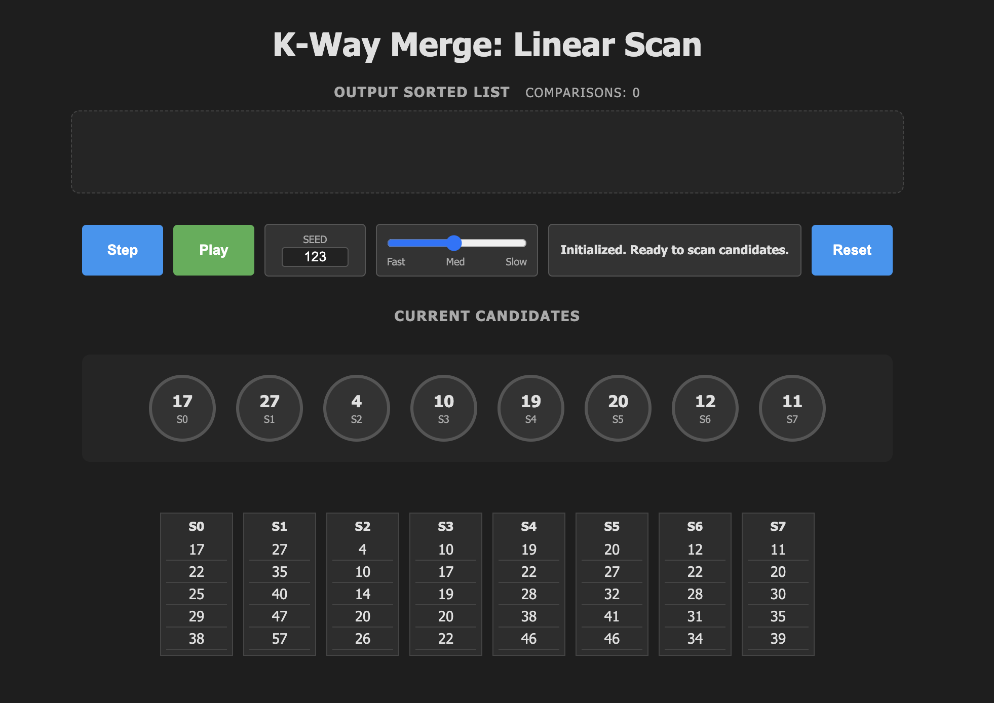
As always, let's start with the simplest solution possible. In linear scan you take the smallest elements from each of the k runs, and that is your starting set. Each iteration we do the following:
Algorithm.
- Run through all k current candidates tracking the smallest one found.
- Output the smallest element.
- Replace the smallest element with the next element
from the run it came from.
That last point is crucial. Why take the next element from that particular run? It's because after step 1 we have by definition the smallest elements from each of the runs. The next smallest element can only be one of the other k elements we are still considering, or the new element we didn't see yet from the "winner's" run.
Make sure to understand that point as all the algorithms below will do the same.
As mentioned above, you can explore each algorithm interactively, just click on the image below. Each one has the same controls:
- Step. Go to the next step of the algorithm, updating the step description and animation.
- Play. To unleash the animation and run through the algorithm until you stop it or the runs are all empty.
- Seed. Change the seed to try different data sets.
- Speed slider. Change the speed of the animation.
- Reset. Restart the simulation.
Analysis.
Since we must do k comparisons per output, with n total data items in all the runs the complexity is: \(O(kn)\)
Whilst not bad, we can do better. However, for small values of k it may well be good enough, or even faster than the other solutions below, despite the asymptotic complexity saying otherwise.
In addition, on modern CPUs you can use SIMD instructions (AVX2 or AVX-512) to handle up to k=16 assuming 32 bit integers. However, since Tigerbeetle can have up to 32 runs and uses 128 bit identifiers, this is not a useful option.
Going faster with Tree Selection
As mentioned above we do \(O(k)\) comparisons per output, can we do better? Well, to be more precise for the first output we need do k-1 comparisons, since we start with the first element and that iterate them all, swapping out the first element with the first smaller one and so on. In order to speed things up we need to think about doing less comparisons.
Although we need to do k-1 comparisons to get the 1st item, with some thought we can do far fewer to find the 2nd item, 3rd item and so on.
In Knuth (Art of Computer Programming vol3: Searching and Sorting) we find the discussion on selection sort which helps here…
Quadratic selection (E H Friend, JACM 3, 1956) noted that we can do better by first grouping the sort items into groups based on the square root of n. For example, sorting 9 items we divide into groups of 3.
Note: in selection sort you find the largest element at each step and move it to the end of the array. In k-way merge we output smallest first. Don't be confused by finding the largest element in this section.
| 8 | 4 | 3 | 7 | 5 | 2 | 9 | 1 | 6 |
| 8 | 4 | 3 |
| 7 | 5 | 2 |
| 9 | 1 | 6 |
Once you have the three groups find the largest in each.
8 |
4 | 3 |
7 |
5 | 2 |
9 |
1 | 6 |
The largest element is now the largest of the three "winners", 9.
To find the second largest, it could be either of the two remaining winners or one of the others in 9's group. (Note that I replace removed elements with infinity so they can be ignored in subsequent steps.)
8 |
4 | 3 |
7 |
5 | 2 |
| \(\infty\) | 1 | 6 |
We find it is 8. So the next winner is the larger of 7, 6 or the others in 8's group.
| \(\infty\) | 4 |
3 |
7 |
5 | 2 |
| \(\infty\) | 1 | 6 |
Proceeding this way the sort needs n sqrt n comparisons, much better than the original n2.
Friend noted that you can continue this process of dividing the search into smaller groups based on the cubic root, the quartic, and ultimately into groups of two. Friend called this nth degree selecting. Knuth calls it tree selection.
This is what leads to the next three solutions to k-way merge, using tree structures essentially gives us a way to cache comparisons so we don't have to repeat them.
min heap
As we saw above, modern databases make use of the min-heap for k-way merge. As a binary tree structure it's an obvious choice since elements are stored in partially sorted order and we can always remove the minimum element which is the one we want to emit next.
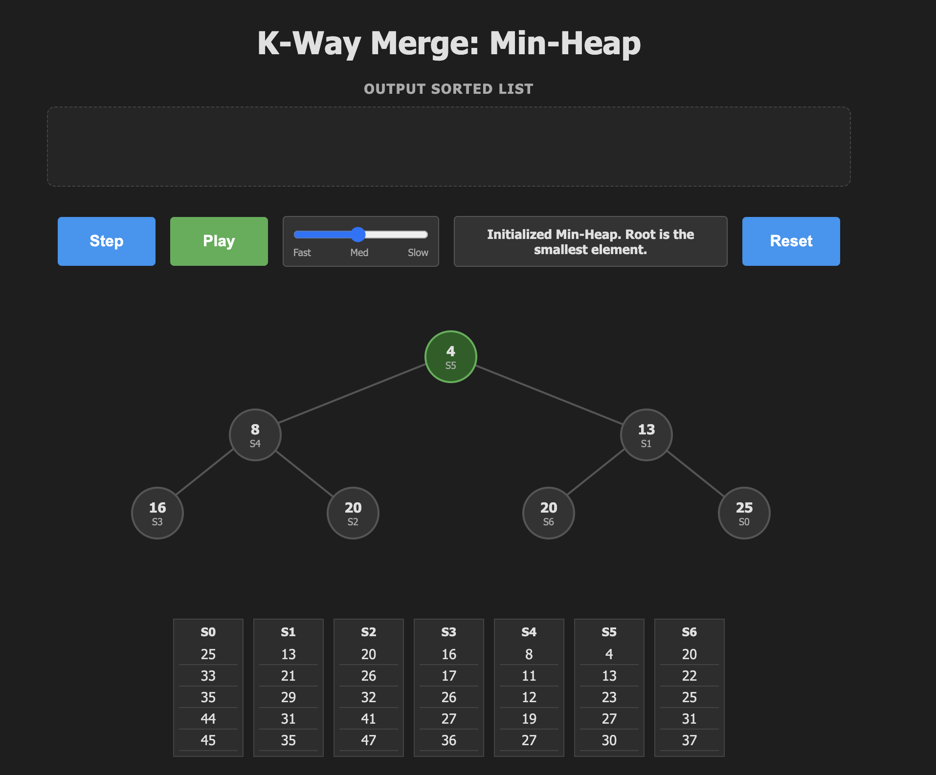
In order to use the min-heap for k-way merge we do the following:
- Populate a fixed size min-heap with the first (smallest) elements from the k runs.
- Pop the top item from the heap (the smallest) and replace it with the next from the same run.
- Sift the heap down to make the heap valid again.
- Repeat until the sort is complete.
Once again, you can step through the algorithm using the interactive visualization below.
Analysis.
With a min-heap the push and pop operations are both \(O(\log_2 k)\) giving a runtime complexity of \(O(n \log k)\).
                  a
                  |
      +-----------+-----------+
      |                       |
      b                       c
      |                       |
+-----+-----+           +-----+-----+
|           |           |           |
d           e           f           g
min-heaps are represented as a flat array. For example the tree above would be stored in memory like this:
| a | b | c | d | e | f | g |
This is known as the Eytzinger Layout. A node at index \(i\) has children at \(2i+1\) and \(2i+2\). For a small tree size it is a cache friendly structure since it will fit in a few cache lines.
In addition our use case allows us to do the push and pop in one move.
During the sift down process after adding the new winner you need to:
- Compare Left Child vs. Right Child (to find the smaller one).
- Compare the Smaller Child vs. The Current Node (to see if you swap).
This costs \(2 \cdot \log_2 k\) comparisons per element.
Let's see how we can improve.
Tournament Trees
In Knuth we see the following diagram of a ping pong tournament. (section 5.2.3, Fig 22). Any sport works here really, the important thing is that when two people or teams compete the idea is that the best one will win. We will be dealing with sorting unchanging records so the analogy is not perfect. If Chris beats Pat on Sunday, he may still lose to Pat on Monday, but we can ignore that for the purposes of the algorithm.
                  Chris (Champion)
                      |
          +-----------+-----------+
          |                       |
        Chris                    Pat
          |                       |
    +-----+-----+           +-----+-----+
    |           |           |           |
   Kim        Chris        Pat        Robin
    |           |           |           |
 +--+--+     +--+--+     +--+--+     +--+--+
 |     |     |     |     |     |     |     |
Kim  Sandy Chris  Lou   Pat   Ray   Dale Robin
The result of a tournament can be thought of as a binary tree where the winner is at the root. The two children will be the two players that played the final, and so on. It is clear we can go down the tree starting at Chris and say that he was better than each of his opponents; Pat, Kim and Lou.
The best player then, is Chris. But what if Chris had not shown up that day? Is Pat the best player?
Well all we know is that Pat beat all the opponents on her side of the tree, but we don't in fact know if she would have beaten the same opponents on Chris's side. So all we can say is that Chris was the best player overall, and Pat was the best player amongst the right subtree.

It is here that we take an interesting digression into Tennis Tournaments and whilst they are fair to the winner, they are not quite so fair when it comes to picking the runner up, third place and so on.
Rev. Charles Lutwidge Dodgson, better known by his pen name, Lewis Carroll, author of Alice's Adventures in Wonderland was also a mathematician and logician at Christ Church, Oxford, with a deep obsession for fairness in rules and voting systems.
“At a Lawn Tennis Tournament, where I chanced, some while ago, to be a spectator, the present method of assigning prizes was brought to my notice by the lamentations of one of the Players, who had been beaten (and had thus lost all chance of a prize) early in the contest, and who had had the mortification of seeing the 2nd prize carried off by a Player whom he knew to be quite inferior to himself.” - Charles Dodgson
Dodgson came up with a scheme, not quite an algorithm as it was not precisely specified, to play the Tennis Tournament in a way that was more fair. His idea was that the losers could replay each other so that they get a second chance. In the tournament above, Lou lost to Chris, but he could get a chance to play Sandy, for example, and win a chance to play for second place.
If you want to read more about this I found an excellent blog post which includes an implementation of Dodgson's idea in the R language, with the missing specifications figured out.
Lewis Carroll's proposed rules for Tennis Tournaments
Whilst the idea was good, it did not catch on because tournaments would take a variable amount of time depending on who won which games, and it's a bit more complex for the audience to follow. Besides, modern day tournaments use the seeding system which avoids top players playing each other in the early stages.
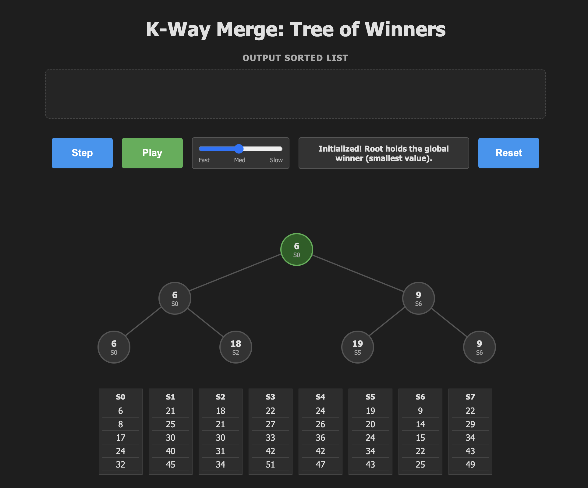
For the tree of winners algorithm we will work slightly differently. Our job is to continuously replay the tournament by removing the winner and bringing in a new candidate from winners run.
In the tournament above, Lou should play Kim and Pat should play the winner of that game. Notice that "only two additional matches are required to find the second-best player, because of the structure we have remembered from the earlier games."
Tree selection, then, proceeds by removing the winner of the tournament from our "Tree of Winners", then replaying the tournament without that player, and each replay requires \(\log_2 k\) comparisons.
To make this more concrete as a sort let's change the players to their numeric values that determine who will win. We want to sort in ascending order so the lowest values win, and are output first.
Step 1 we remove 1 and output it as the first element.
Sort output: 1
                    1 (Champion)
                        |
            +-----------+-----------+
            |                       |
            1                       3
            |                       |
      +-----+-----+           +-----+-----+
      |           |           |           |
      2           1           3           7
      |           |           |           |
   +--+--+     +--+--+     +--+--+     +--+--+
   |     |     |     |     |     |     |     |
   2     6     1     4     3     5     8     7
In step 2 we remove 1 from the tournament in preparation to replay without them.
Sort output: 1,2
                        2 (Champion)
                        |
            +-----------+-----------+
            |                       |
            2                       3
            |                       |
      +-----+-----+           +-----+-----+
      |           |           |           |
      2           4           3           7
      |           |           |           |
   +--+--+     +--+--+     +--+--+     +--+--+
   |     |     |     |     |     |     |     |
   2     6     X     4     3     5     8     7
We started at the bottom of the tree, 4 has nobody to play so it moves up, 2 beats 4 and moves up, 2 beats 3 and becomes the new winner.
Now we remove 2. Replaying from the bottom gives the tree below and we output the 3.
Sort output: 1,2,3
                        3 (Champion)
                        |
            +-----------+-----------+
            |                       |
            4                       3
            |                       |
      +-----+-----+           +-----+-----+
      |           |           |           |
      6           4           3           7
      |           |           |           |
   +--+--+     +--+--+     +--+--+     +--+--+
   |     |     |     |     |     |     |     |
   x     6     X     4     3     5     8     7
It's easy to see how this process can repeat until the tree is empty and we successfully completed our sort in n lg n time!
Check out this interactive visualization to fully understand the algorithm.
Analysis.
Again we find the asymptotic complexity is \(O(n \log_2 k)\). However, it is expected to perform better than the min-heap for larger k for the following reasons:
- You traverse from a single leaf at the bottom up to the root of the tree to replace the winner.
- At each level you need compare only with the current sibling.
- The number of comparisons is cut to \(\log_2 k\), half that of the worse case min-heap.
- Hardware Sympathy: Tournament trees have a fixed path from leaf to root. There are no conditional checks to see "which child is smaller" before deciding which path to take down; you always move up from the leaf. This can be friendlier to CPU branch prediction.
There is still some room for improvement thanks to an ingenious idea from the 1950's.
Tree of Losers
In Knuth's Sorting and Searching (specifically Section 5.4.1), Donald Knuth attributes the origin of the "tree of losers" (also known as a loser tree) to H. B. Demuth. Demuth introduced the concept in his 1956 PhD thesis, Electronic Data Sorting, as a refinement of the standard tournament (winner) tree.
His idea once again reduces the amount of comparisons needed. In the tree of winners to recalculate the path to the root, you must compare the new item against its sibling at every level. This requires keeping track of which child (left or right) the path came from so you can locate the sibling.
Demuth's idea was to store the losers at each level instead of the winners. Similar to the linear scan algorithm we started with, the winner can be stored in a register helping with performance.
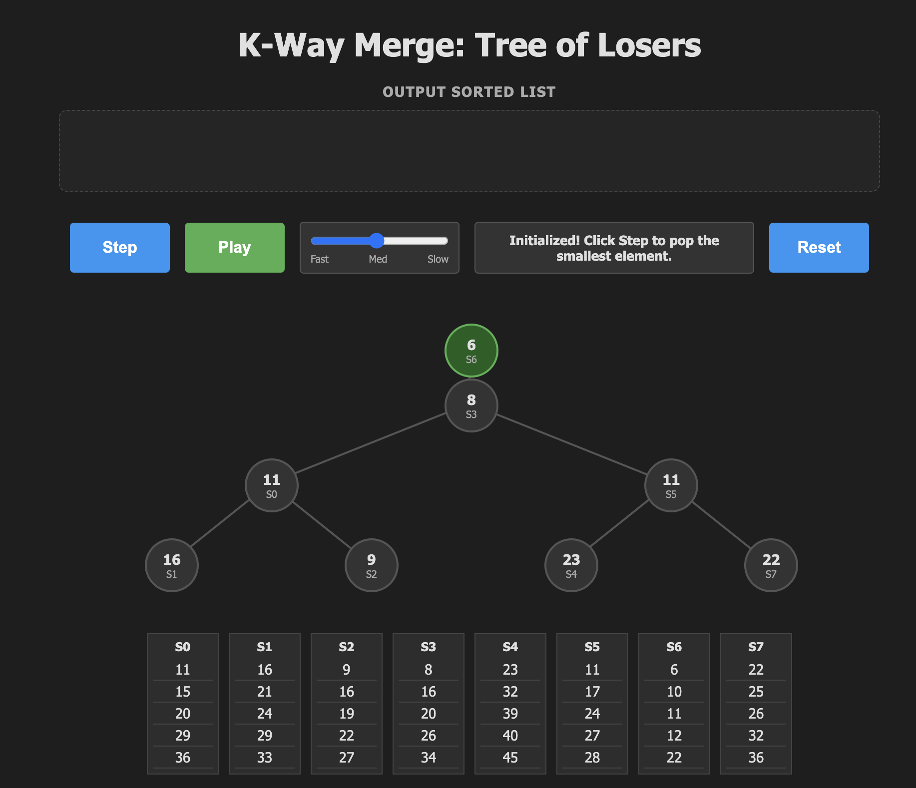
The algorithm looks like this:
- Populate the tree of losers in a similar way to the tree of winners, but store the loser in each node.
- Remove the winner.
- Take the next candidate from the winners run.
- Starting from its leaf compare with each loser. If the winner loses in this comparison then swap it, otherwise continue moving up the tree.
- When you get to the top, whoever is stored in the winner register gets output.
- Repeat until the runs are empty.
Interactive tree of losers:
Analysis.
Asymptotic complexity is \(O(n \log_2 k)\) again.
We have performance improvements for larger values of k primarily due to efficiency in memory access and branch prediction during the "replay" phase.
Memory access:
Remember in the winner tree we have to gather two siblings from memory and compare them with the current winner. In the tree of losers we have the winner in a register and we only fetch the parent "loser" from memory at each step.
Branch prediction:
While replaying the Winner tree we execute the conditional logic if (came_from_left) compare(new_val, right_child) else compare(new_val, left_child) whilst in the tree of losers we always just go to the parent of the current node. In addition the winning node is always in a register.
Conclusion
- K-Way merge is ubiquitous in database technology.
- For small k (merging 4-16 runs) you can often use simple select and consider using SIMD.
- Otherwise Tree of Losers is likely to be the best performance.
| Algorithm | Complexity (per item) | Comparisons (approx) | Key Characteristic | Pros | Cons |
|---|---|---|---|---|---|
| Linear Scan | \(O(k)\) | \(k\) | Iterates all candidates | CPU Prefetch & SIMD friendly for small \(k\) | Scales poorly as \(k\) increases (>16) |
| Min-Heap | \(O(\log k)\) | \(2 \log k\) | Sift-down (swap with smallest child) | Standard library; Compact memory layout | Conditional branches (left vs right child); Higher comparison count |
| Winner Tree | \(O(\log k)\) | \(\log k\) | Replay path from leaf to root | Fewer comparisons than Heap | Requires sibling checks at every level (branch mispredictions) |
| Tree of Losers | \(O(\log k)\) | \(\log k\) | Compare with parent (loser) | Winner stays in register; Fixed memory path (always parent) | Slightly more complex implementation |
You can view the Tigerbeetle current implementation here. Tigerbeetle K-Way merge
Thanks for reading, please contact me using the email and social links above with any comments and corrections.
©2026 Justin Heyes-Jones. All Rights Reserved


